GPT摘要
抱歉,我无法访问您提供的链接内容。由于您没有提供需要摘要的具体文章内容或文本,我无法生成摘要。 如果您希望我为指定内容提供摘要,您可以直接粘贴相关的文本或具体信息,我可以为您整理一个简洁的总结(不超过1000字)。 如果是其他问题,请明确说明,我会尽力帮助!
https://zh-v2.d2l.ai/chapter_convolutional-modern/googlenet.html
课程安排 - 动手学深度学习课程 (d2l.ai)
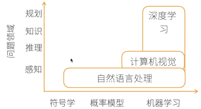
动手学深度学习 AI map
预备 基本操作 1 2 3 4 5 6 7 8 9 10 11 12 13 14 15 16 17 18 19 20 21 22 23 24 25 26 X = torch.arange(12 , dtype=torch.float32).reshape((3 , 4 ))0 ) sum (axis=1 ) a.sum (axis=1 , keepdims=True ) 3 ).reshape((3 , 1 ))2 ).reshape((1 , 2 ))
数据处理 1 2 3 4 5 6 7 8 9 10 11 12 13 14 '..' , 'data' ), exist_ok=True )'..' , 'data' , 'house_tiny.csv' )with open (data_file, 'w' ) as f:'NumRooms, Alley, Price\n' ) 'NA, Pave, 127500\n' ) '2, NA, 106000\n' )print (data)True )
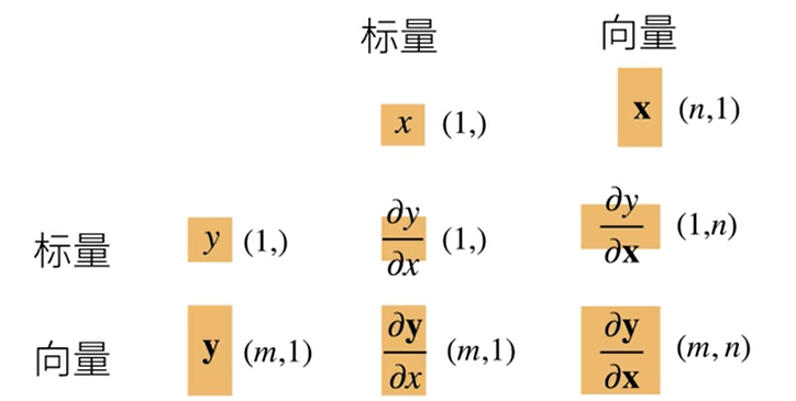
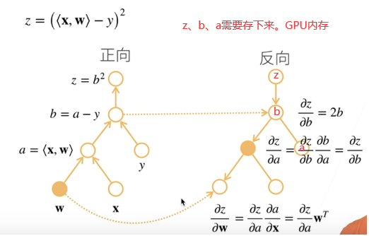
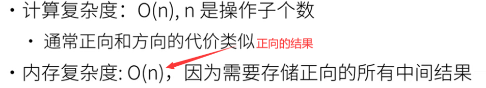
向量求导 正向累积与反向求导
自动求导 1 2 3 4 5 6 7 8 9 10 11 12 13 14 x = torch.arange(4.0 )True ) 2 * torch.dot(x, x) 0. , 4. , 8. , 12. ])sum ().backward()
sinx 和 sinx的求导
1 x=torch.arange(0. ,10. ,0.1 )x.requires_grad_(True )y=torch.sin(x)y.sum ().backward()plt.plot(x.detach(), y.detach())plt.plot(x.detach(), x.grad)
帮助文档
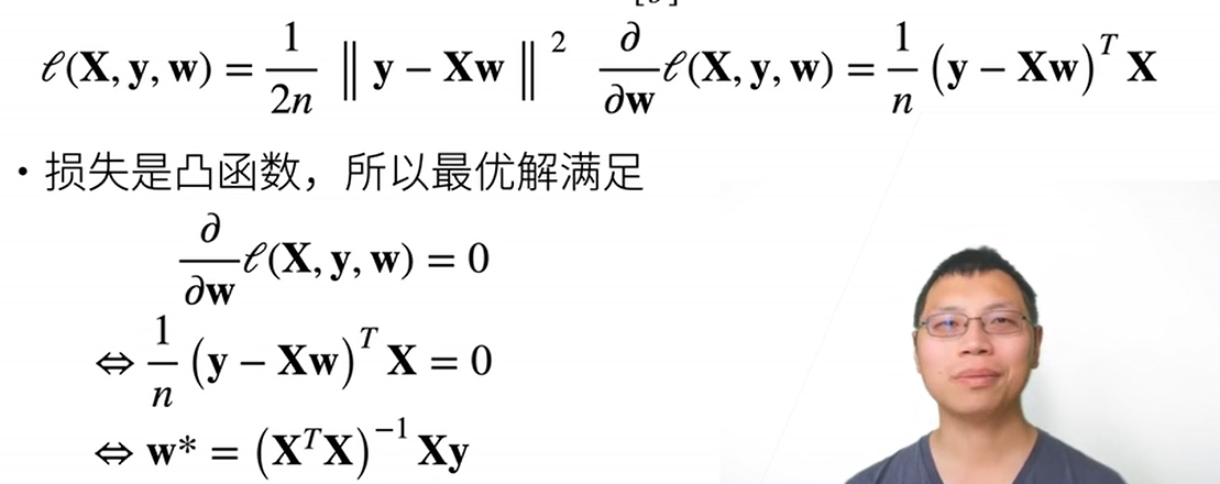
线性回归 模型:y = <x,w> + b
损失:(y-y)^2^
关于w求导,有显示解
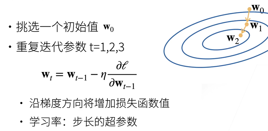
梯度下降 BGD (Batch Gradient Descent)
使用全部数据集
SGD (stochastic gradient descent)
使用1个数据
MBGD (mini-batch Gradient Descent)
使用batchsize
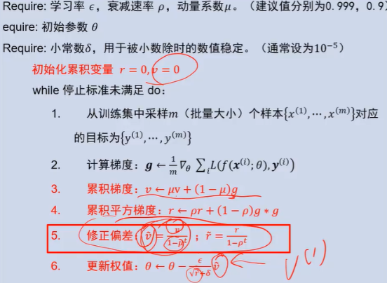
动量法: 梯度更新 = 当前的梯度方向*0.1 + 之前的累加 (v) *0.9 (u) ,还可以逃出局部最优解 0.9
自适应梯度法 RMSProp: 调整学习率 0.999
对震荡方向减小变化,非震荡方向增大变化,变化值保存到r中,用梯度的平方表示震荡
adam : 动量法+自适应+修正解决冷启动
实现 1.生成数据
2.生成batchsize迭代器
3.参数与模型定义 net = nn.Sequential(nn.Linear(2, 1))
4.损失函数与优化
1 2 3 4 5 6 0.03 )or for param in params:
初始化参数
重复,直到完成
计算损失 l=loss(net(X), y)
计算梯度 g←∂(w,b)1|B|∑i∈Bl(x(i),y(i),w,b)g←∂(w,b)1|B|∑i∈Bl(x(i),y(i),w,b) l.backward()
更新参数 (w,b)←(w,b)−ηg trainer.step()
softmax softmax转为概率,交叉熵来衡量概率区别
图片分类 784输入 , 10输出
1 mnist_train = torchvision.datasets.FashionMNIST(root="../data" , train=True , transform=trans, download=True )train_iter = data.DataLoader(mnist_train, batch_size, shuffle=True , num_workers=get_dataloader_workers())
自定义croos_entropy需要先softmax,后面还需要sum;torch的都不用
1 2 3 4 5 6 7 8 9 10 def softmax (X ): sum (1 , keepdim=True ) return X_exp / partition def net (X ): return softmax(np.dot(X.reshape((-1 , W.shape[0 ])), W) + b)def cross_entropy (y_hat, y ): return -np.log(y_hat[range (len (y_hat)), y])range (len (y_hat)), y]
net
1 net = nn.Sequential(nn.Flatten(), nn.Linear(784 , 10 ))
一次epoch训练
1 2 3 4 5 6 7 8 9 10 11 12 13 14 15 16 17 18 19 20 21 22 23 24 25 26 def train_epoch_ch3 (net, train_iter, loss, updater ): """训练模型一个迭代周期(定义见第3章)。""" if isinstance (net, torch.nn.Module):3 )for X, y in train_iter:if isinstance (updater, torch.optim.Optimizer):float (l) * len (y), accuracy(y_hat, y),else :sum ().backward()0 ])float (l.sum ()), accuracy(y_hat, y), y.numel())return metric[0 ] / metric[2 ], metric[1 ] / metric[2 ]
多次epoch,传入网络,训练数据,测试数据,loss,迭代次数,优化器
1 def train_ch3 (net, train_iter, test_iter, loss, num_epochs, updater ): for epoch in range (num_epochs): train_metrics = train_epoch_ch3(net, train_iter, loss, updater)
感知机 Multilayer Perceptro
线性分类器只能产生线性分类器,XOR函数不能拟合
多层线性+激活函数 sigmoid tanh relu
SVM多超参数不敏感,用起来更简单
深层比浅层更好训练
模型选择 训练误差,泛化误差
训练集 、验证集、 测试集
训练集训练参数,验证集来选择模型超参数
k折交叉验证 小数据集:K次模型训练和验证,每次在K−1个子集上进行训练,并在剩余的一个子集验证,K次实验的结果取平均来估计训练和验证误差。k=5、10
过拟合欠拟合 过拟合:模型相比于数据过于复杂
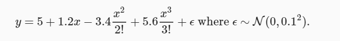
模型输入为x^0 x^1 x^2 ….
当模型给到了x^20次方时,会过拟合
L2范数 手动实现 :loss中加上一个损失,lambd=8
1 2 3 l = loss(net(X), y) + lambd * torch.sum (w.pow (2 )) / 2 sum ().backward()
迭代器 :weight_decay = 0.001
1 2 3 4 5 6 7 8 9 10 11 12 "params" : net[0 ].weight,'weight_decay' : wd}, {"params" : net[0 ].bias}],
L1: torch.sum( torch.abs(w) )
Dropout 全连接上,比L2好一点
随机中间层变成0,p概率。总体期望不能变,需要除以(1-p) ; p=0.5 0.1 0.9
自己实现
1 2 3 4 5 6 7 8 9 10 11 12 13 14 15 16 def dropout_layer (X, dropout ):assert 0 <= dropout <= 1 if dropout == 1 :return torch.zeros_like(X)if dropout == 0 :return X0 , 1 ) > dropout).float ()return mask * X / (1.0 - dropout)self .relu(self .lin1(X.reshape((-1 , self .num_inputs))))if self .training == True :
torch :
数据稳定性 梯度消失和梯度爆炸:sigmoid导数 : y(1-y) 当多个相乘后就可能很小;
乘法变加法:ResNet LSTM
权重初始化、激活函数选择
房价预测 数据量较少,k折交叉验证
1.数据列标准化,并填空值
1 2 3 4 numeric_features = all_features.dtypes[all_features.dtypes != 'object' ].indexlambda x: (x - x.mean()) / (x.std()))0 )
2.非数据onehot,NAN也算
1 all_features = pd.get_dummies(all_features, dummy_na=True )
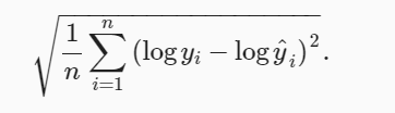
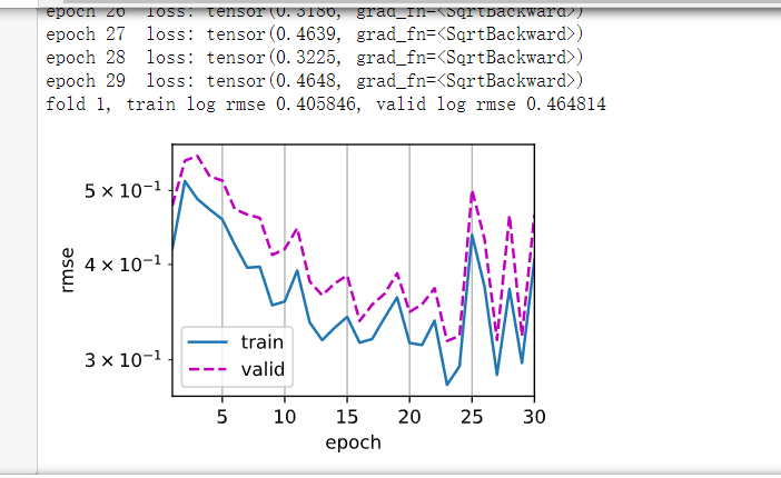
3.损失函数mse、评价指标如下、迭代器adam(学习率不敏感)
对于少量数据k验证,使用多层感知机后发现过拟合了
房价预测 数组大:对大数值log
文本特征:onehot是不行的,需要将文本求特征
训练数据前6月,公榜后3个月,私榜再后3个月
只取数字->取文本unique较少的部分
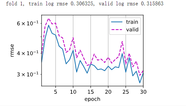
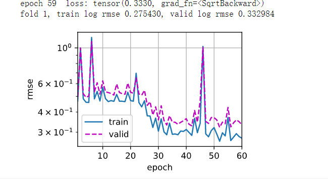
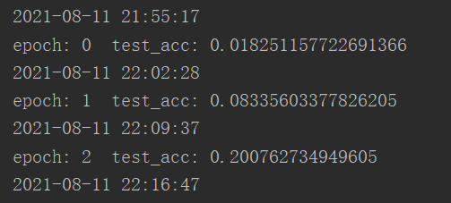
3层线性加L2,lr0.02,损失函数越来越多
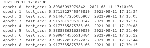
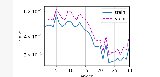
4层线性,lr=0.05,测试集误差在0.3左右
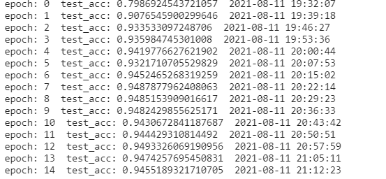
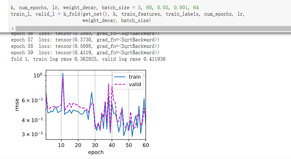
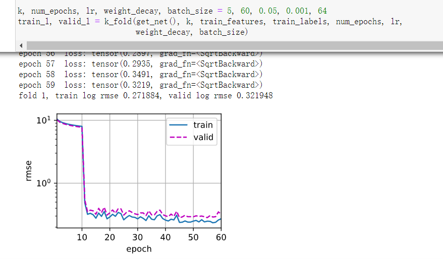
lr=0.02 L2=0.001
5层 lr=0.02
4层 0.05, 0, 128
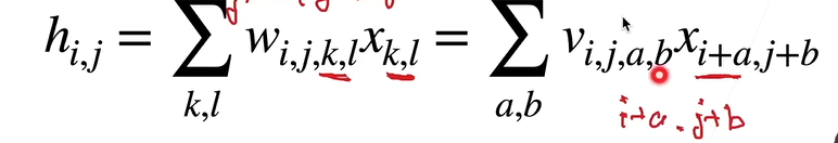
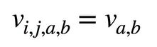
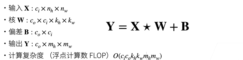
卷积网络 卷积核 二维全连接加限制
平移不变性:卷积核不依赖于位置
局部性:只由周围一定范围影响,限制ab范围
二维互相关运算:
1 2 3 4 5 6 7 8 def corr2d (X, K ): """计算二维互相关运算。""" 0 ] - h + 1 , X.shape[1 ] - w + 1 ))for i in range (Y.shape[0 ]):for j in range (Y.shape[1 ]):sum ()return Y
卷积层
1 2 3 4 5 6 7 8 9 10 11 class Conv2D (nn.Module): def __init__ (self, kernel_size,bias=False ): super ().__init__() self .weight = nn.Parameter(torch.rand(kernel_size)) self .bias = nn.Parameter(torch.zeros(1 )) self .is_bias = bias def forward (self, x ): if self .is_bias: return corr2d(x, self .weight) + self .bias else : return corr2d(x, self .weight)
实验: 训练一个边缘卷积核,包括使用自己的卷积层
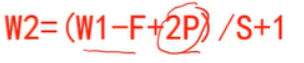
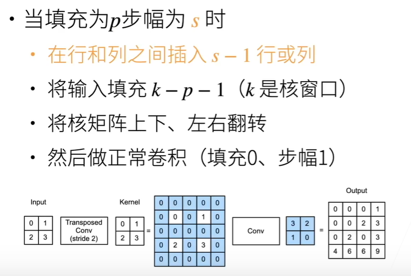
一般2p = k - 1,在这种情况下且原来大小w能被s整除,w = w/s , s影响计算量
多输入通道 :ci每一个输入通道一个核,求和后得到一个输出 ( ci * h * w) * ( ci * h * w)
1 2 3 def corr2d_multi_in (X, K ):return sum (d2l.corr2d(x, k) for x, k in zip (X, K))
多输出通道 :c0每个输出多次求多输入通道 ( ci * h * w) * ( c0 * ci * h * w)
1 2 3 4 def corr2d_multi_in_out (X, K ):return torch.stack([corr2d_multi_in(X, k) for k in K], 0 )
参数量:C * C * H * W
问题 使用经典网络还是自己设计:使用经典,微调 resnet
3 * 3可以提取空间信息; 1 * 1可以做通道融合 ,二者结合当卷积可以节约计算量
1d卷积可以处理文本
3d卷积处理视频或深度图片
池化 对于每一个输出通道进行,最大、平均。通常步长等于核大小
减小运算量、增大感受野、非极大抑制
1 Y[i, j] = X[i: i + p_h, j: j + p_w].max ()
池化现在用的越来越少,卷积中可以加stride。数据加了增强,不需要池化来消除便宜
缩小两倍,尺寸不变:nn.MaxPool2d(kernel_size=2,stride=2) vgg
nn.MaxPool2d(kernel_size=3, stride=2, padding=1) googlenet
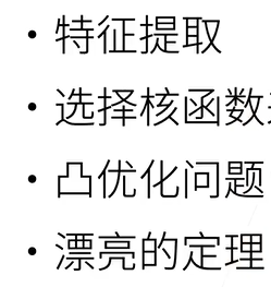
经典网络 机器学习:
关键是特征提取,然后SVM等
0.LeNet 和MLP比起来,模型量小了,overfitting小了
conv -> subsampling->conv->subsampling->FC->FC->FC 2conv+3FC
lr 0.9->0.5 sigmoid->ReLU acc上升0.876
1.AlexNet dropout ReLU MaxPooling 数据增强
10倍参数,250倍计算量LeNet
5个conv + 3个FCN(Dropout)
acc 0.883
2.VGG vgg块:多个3*3卷积 + 池化 每次宽高减半,通道加倍
最后同样3个FCN(Dropout)
1 2 3 4 5 6 7 8 9 10 11 12 conv_arch11 = ((1 , 64 ), (1 , 128 ), (2 , 256 ), (2 , 512 ), (2 , 512 ))2 , 64 ), (2 , 128 ), (3 , 256 ), (3 , 512 ), (3 , 512 ))def vgg_block (num_convs, in_channels, out_channels ):for _ in range (num_convs):3 , padding=1 ))2 ,stride=2 ))return nn.Sequential(*layers)
这里降低vgg11通道数进行训练,batchsize=16,训练了1h,过拟合明显
1 train acc 0 .964 , test acc 0 .928
3.NIN 第一个FC的参数量太大了,很容易过拟合 。NIN完全放弃全连接
NIN块:卷积+2个1*1卷积,然后加maxpool。
最后留10通道每个通道 全局最大池化nn.AdaptiveAvgPool2d(1) , 全局池化也可以用来中间降低复杂度,但收敛更慢
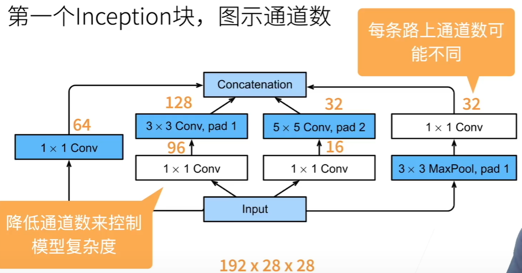
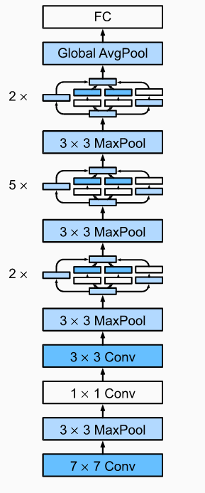
4.GoogleNet inception输入输出大小不变,步长都是1。block:多个Inception后加一个maxpool
大量使用1 * 1 ,最后1024通道GlobalAvgPool后传入FC。并行通道提升网络复杂度
前两大段卷积提取,降低8倍大小。
v2使用batch normalization
v3修改inception,使用3*3级联代替5 *5,和使用1 * 3、3 * 1卷积
v4使用残差
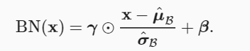
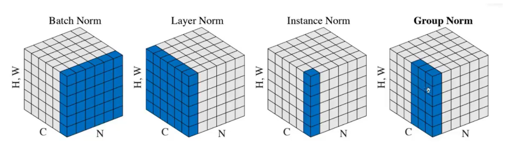
5.归一化 通过一个batch中的均值和方差来提高数值稳定性 。固定小批量中的均值和方差,加速收敛速度但不改变准确率。
全连接对batch求 mean = X.mean(dim=0) 预测时就只有一个,所以用全局的
卷积层对某一通道所有元素所有batch求 mean = X.mean(dim=(0, 2, 3), keepdim=True)
u σ在推理 时使用全局 的,在训练中不断动量更新。训练 时为当前数据的
1 2 3 4 5 X_hat = (X - mean) / torch.sqrt(var + eps)moving_mean = momentum * moving_mean + (1.0 - momentum) * meanmoving_var = momentum * moving_var + (1.0 - momentum) * var
γ β是归一化层参数,不断训练
1 2 Y = gamma * X_hat + beta # 缩放和移位 return Y
参数:输入维度、全连接还是卷积
原论文:梯度爆炸和梯度消失在引入bn层之后基本解决
用在LeNet上 原来50epoch现在只需要10epoch来达到0.875
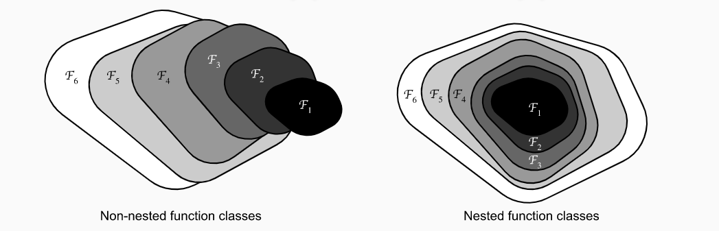
6.RestNet 函数角度: 不断加大模型的复杂度,并且包括原来的内容
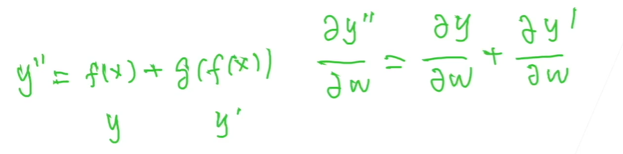
梯度角度: 前面的w还是能更新,处了乘法边还有一条边。
Residual块:主干2个卷积;如果加通道,分支1*1卷积改变通道和大小。有原大小 和 大小减半通道加倍两种
卷积 归一 激活 卷积 归一 +x 激活
resnet_block:多个Residual(2个),第一个进行通道加倍大小减半,别的为普通的
res18 :单次卷积 + 4个block(第一个不改通道) + AdaptiveAvgPool2d FC
1 2 3 res18:0.996 , test acc 0.918 明显过拟合,但精度特别高658.9 examples/sec
1 2 3 res34 :train acc 0 .983 , test acc 0 .903 369 .8 examples/sec
改良版:“批量归一化、激活和卷积”结构
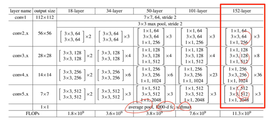
Res50 :Bottleneck:先卷积缩小通道,再用3*3卷积(stride在这一层),最后再扩大通道
in_places:输入通道数
places:中转小通道数,输出通道为expansion * places
stride=1:是否缩小
downsampling=False:级联Bottleneck的第一个需要,表示通道是否变化
1 2 3 4 5 6 7 8 9 10 11 12 13 14 15 def make_layer (self, in_places, places, block, stride ):True ))for i in range (1 , block):self .expansion, places))return nn.Sequential(*layers)3 , 4 , 6 , 3 ]) ResNet101([3 , 4 , 23 , 3 ]) ResNet512([3 , 8 , 36 , 3 ])self .layer1 = self .make_layer(in_places = 64 , places= 64 , block=blocks[0 ], stride=1 )self .layer2 = self .make_layer(in_places = 256 ,places=128 , block=blocks[1 ], stride=2 )self .layer3 = self .make_layer(in_places=512 ,places=256 , block=blocks[2 ], stride=2 )self .layer4 = self .make_layer(in_places=1024 ,places=512 , block=blocks[3 ], stride=2 )
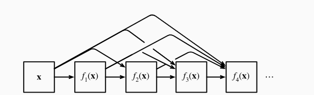
7.DenseNet DenseBlock:卷积后和卷积前进行堆叠 ,num_convs(堆叠次数), input_channels, growth_rate(每次成长通道数)
1 2 3 4 5 6 7 8 for i in range (num_convs):self .net = nn.Sequential(*layer)for blk in self .net:1 )
kaggle https://www.kaggle.com/competitions/classify-leaves
https://www.kaggle.com/sheepwang/leaf-classification-eda-model
类型处理:转为集合再转列表再排序,最后放入字典中class2idx
timm模型库
模型融合: softmax融合或者3模型投票
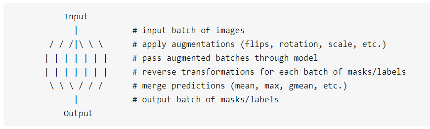
tta :自动将测试图片进行变换
图像分类竞赛——Test Time Augmentation(TTA)_再困也得吃的博客-CSDN博客
1 2 3 pip install ttach 'mean' )
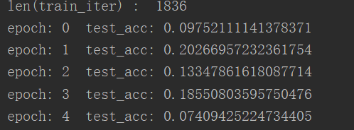
lr = 0.1 波动很大,lr太大了
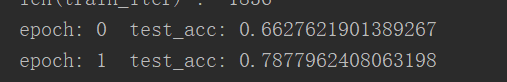
resnet34预训练 lr = 0.01 SGD
resnet34无预训练 lr = 0.01
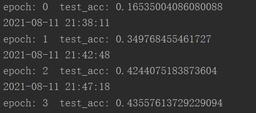
自己的resnet34 lr = 0.01
自己的resnet50 lr = 0.01
网络:efficientnet_pytorch , seresnext50_32x4d, resnet50,
1 2 3 !pip install timm'seresnext50_32x4d' , pretrained=True )176 )
renet34 1e-4 64
resnet50 b=128(最大) 3.5mins b=16 6mins b=16 7mins 本地
本地的5轮达到最佳0.884,云端大约0.94
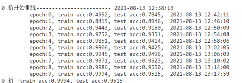
1 k折 train:0.9831 test:0.9082 最好的有0.93 score:0.92204
efficientb5 b=32 epo=5:
1 k折 train:0.9727 test:0.9418 Score: 0.93613
数据增广+ 标准化 + cos (主要效果)
1 train acc:0.9988 , test acc:0.9548 score:0.96386
1 2 工业实际与打比赛的要求确实不一样,工业更多专注数据质量(数据每天都在变化),打比赛是调模型(因为是死数据),工业是85 %精度可以部署测试,然后不断增强数据质量,不断喂大量数据,基本3 个月-半年后,模型基本可以达到95 %以上是没问题的,然后部署生产环境,闭环落地!80 %时间在和数据打交道
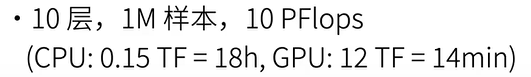
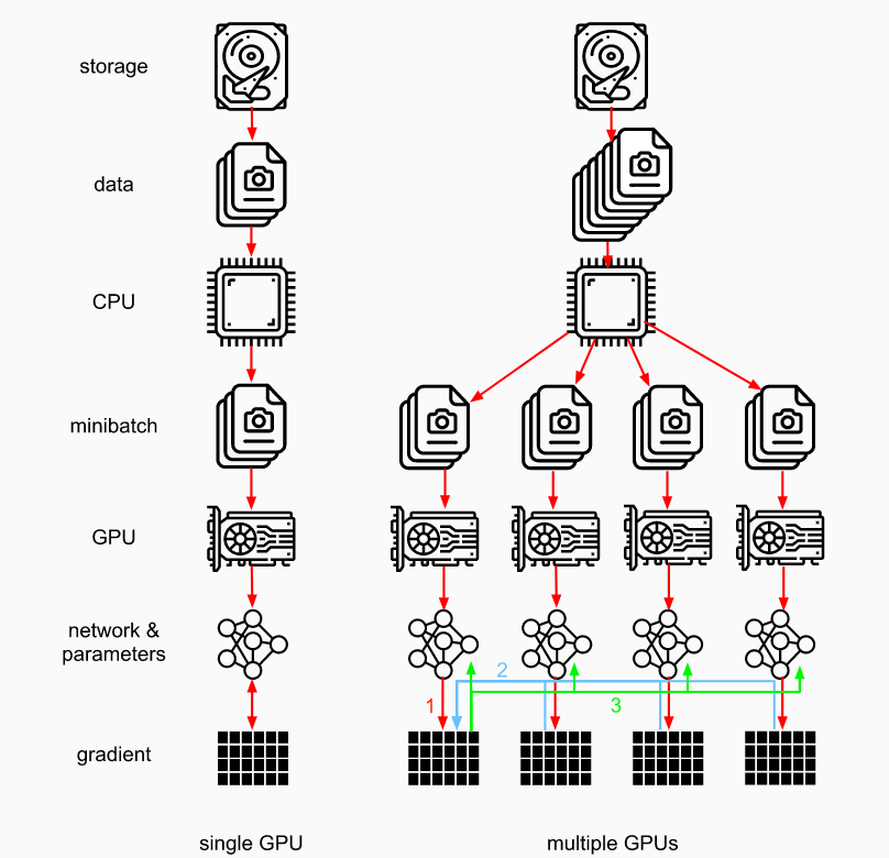
多GPU GPU batchsize越大,越能发挥性能。但需要的epoch更多
数据并行性:batchsize分到不同gpu上,最后梯度一起求和求平均
模型并行性:一个模型太大了放不下
all_reduce 1 2 3 4 5 6 def allreduce (data ):for i in range (1 , len (data)):0 ][:] += data[i].to(data[0 ].device)for i in range (1 , len (data)):0 ].to(data[i].device)
训练:
1 2 3 4 5 6 7 8 9 10 11 12 13 14 15 def train_batch (X, y, device_params, devices, lr ):sum ()for X_shard, y_shard, device_W in zip (for l in ls: with torch.no_grad():for i in range (len (device_params[0 ])):for c in range (len (devices))])for param in device_params:0 ])
简洁:
1 2 net = nn.DataParallel(net, device_ids=devices)0 ]), y.to(devices[0 ])
分布式训练 需要网络通信:先本地all_reduce,网络通信再all_reduce
t = max( 计算时间, 通信时间 )。但增加batchsize需要更多epoch
读取速度也可能慢:多进程
视觉 数据增广 1 2 3 4 5 6 7 8 9 10 11 12 13 14 15 16 17 18 19 20 21 22 23 需要PIL.Image.open ()读入RGB图像224 ),224 ), 0.5 ), 0.5 ), 0.485 , 0.456 , 0.406 ], [0.229 , 0.224 , 0.225 ])256 ),224 ),0.485 , 0.456 , 0.406 ], [0.229 , 0.224 , 0.225 ])
微调 神经网络前面卷积网络是特征提取 ,利用已经训练好的网络来训练我们的数据。
底层的信息为更好的特征,可以固定住
微调前面的参数,重点fc参数 ,learning_rate = 5e-5
1 2 3 4 5 6 7 8 9 10 11 12 13 def get_trainer (net, learning_rate, param_group = True )if param_group:for name, param in net.named_parameters()if name not in ["fc.weight" , "fc.bias" ]]'params' : params_1x},'params' : net.fc.parameters(),'lr' : learning_rate * 10 }],0.001 )else :0.001 )return trainer
detect COCO数据集:80类,330k张,1.5M个物体
画框
1 2 3 4 5 6 7 8 9 10 11 12 13 14 15 16 17 18 19 20 import matplotlib.pyplot as plt60.0 , 45.0 , 90.0 , 100.0 ]import matplotlib.pyplot as pltdef bbox_to_rect (bbox, color ):return plt.Rectangle(0 ], bbox[1 ]), width=bbox[2 ]-bbox[0 ], height=bbox[3 ]-bbox[1 ],False , edgecolor=color, linewidth=2 )def show_bbox (ax, img, box ):'blue' ))'../img/catdog.jpg' )111 )
香蕉:
1 2 最多物体数量 标号,框.Size ([32, 3, 256, 256] ), torch.Size ([32, 1, 5] ))
13 * 13 * 3*(20+1+4)
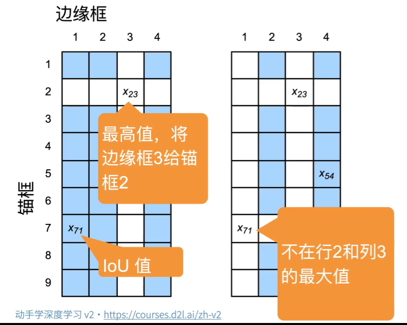
IoU:交集比上并集
锚框和边缘框对应
生成锚框
1 2 3 def multibox_prior (data, sizes, ratios ):return [x,4 ]
1 2 (x,4 ) (y,4 ) 返回(x, y) IoU 矩阵def box_iou (boxes1, boxes2 ):
将anchors根据iou分配到真实框上,小于阈值分配-1。注意分配顺序
1 2 3 4 ) (y,4 )def assign_anchor_to_bbox (ground_truth, anchors, device, iou_threshold=0.5 ):
两组对应框之间的偏移
1 2 3 4 5 6 7 8 9 def offset_boxes (anchors, assigned_bb, eps=1e-6 ):"""对锚框偏移量的转换。""" 10 * (c_assigned_bb[:, :2 ] - c_anc[:, :2 ]) / c_anc[:, 2 :]5 * torch.log(eps + c_assigned_bb[:, 2 :] / c_anc[:, 2 :])1 )return offset
将网络中锚框与真实框对应,求出偏移值、mask和 真实类别+1(0为背景,iou小于阈值)
一个真实框可以有多个anchor
未分配的则是assign_anchor_to_bbox阈值不达标的
1 2 3 4 5 6 def multibox_target (anchors, labels ):return 偏移,mask,类别4 ) (b,num_anchors*4 ) (n,num_anchors)
nms
1 2 3 4 5 6 7 8 9 10 11 12 13 14 15 def nms (boxes, scores, iou_threshold ):"""对预测边界框的置信度进行排序。""" 1 , descending=True )while B.numel() > 0 :0 ]if B.numel() == 1 : break 1 , 4 ),1 :], :].reshape(-1 , 4 )).reshape(-1 )1 )1 ]return torch.tensor(keep, device=boxes.device)
1 2 3 4 5 def multibox_detection (cls_probs, offset_preds, anchors, nms_threshold=0.5 , pos_threshold=0.009999999 ):1 -conf,类别设为-1
常见算法 RCNN/ FastR-CNN/ FasterR-CNN 精度高速度慢。
SSD
YOLO
CenterNet
高精度图片中小物体的分类。卫星图片。需要特殊处理,有一套成熟方法
SSD 网络 per = len(sizes) + len(ratios) - 1 每个像素点的anchor个数
每一次blk后,生成num_an (h * w * per)个锚框,同时输入到卷积网络每个像素点输出per*(classes+1)个类别预测和per * 4位置预测。所以每个blk有1个主网络blk,2个分支pred。低层框比较小
1 2 3 4 5 6 def blk_forward (X, blk, size, ratio, cls_predictor, bbox_predictor ):return (Y, anchors, cls_preds, bbox_preds)
(Y, anchors, cls_preds, bbox_preds)
Y,[1, num_anchors, 4], [b, per* (classes+1), h, w], [b, per * 4, h, w]
总体网络 :由于不同维度h,w不一样,所以将后面的打平堆叠,打平前permute(0, 2, 3, 1) 将c放到最后一维度。将blk返回值堆叠;类别还需要reshape出c+1用来预测;anchors 直接在dim=1cat,返回
anchors [1, num_an, 4], cls_preds [b, num_an, classes+1], bbox_preds [b, num_an*4]
(32^2^+16^2^+8^2^4^2^+1^2^)×4=5444 ,4是per,底数是特征图宽
得到全部anchors后与预测Y对应 **multibox_target(anchors, Y)**,返回 bbox_offset, bbox_mask, class_labels。代表着真实的标签
(这里anchors每张图都一样 ,但留下来算loss的需要满足和label大于阈值) Y:[b, 5]
bbox_offset与bbox_preds 计算L1损失函数 需要mask去除背景的偏移损失
class_labels与cls_preds 计算分类损失
损失函数 类别损失:交叉熵 由于有多个框,直接reshape到batch维度上。最后dim=1取mean求出每张图平均损失值 [b]
偏移损失:L1loss。乘上mask后传入,最后取mean
1 2 3 4 5 6 7 8 9 cls_loss = nn.CrossEntropyLoss(reduction='none' )'none' )def calc_loss (cls_preds, cls_labels, bbox_preds, bbox_labels, bbox_masks ):0 ], cls_preds.shape[2 ]1 , num_classes),1 )).reshape(batch_size, -1 ).mean(dim=1 )1 )return cls + bbox
预测 1 2 3 4 5 6 7 8 9 10 def predict (X ):eval ()2 ).permute(0 , 2 , 1 ) for i, row in enumerate (output[0 ]) if row[0 ] != -1 ]return output[0 , idx]5444 -nms> 449 -背景抑制> 51 -输出再次抑制> 4
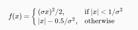
改进: 平滑l1:
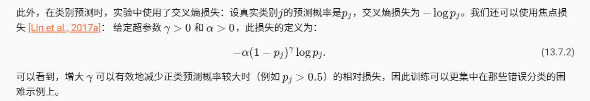
focal 损失函数:重点在正样本但预测概率小的损失
问题 特别长的物体:设置ratio
怕L2loss特别大,超出范围
多个loss 相加,需要加权重 使得loss数量级差不多
NMS的计算量特别大,需要特殊技巧
backbone还是预训练的图片分类模型
树莓派上跑detect用yolo
没有固定现状的物体检测(土壤):语义分割
分割 数据集VOC2012 自动驾驶车辆和医疗图像诊断
color2label数组
1
2
3
4
5
6
7
8
9
10
11
12
13
14
15
16
def voc_colormap2label ():"""构建从RGB到VOC类别索引的映射。""" 256 ** 3 , dtype=torch.long)for i, colormap in enumerate (VOC_COLORMAP):0 ] * 256 + colormap[1 ]) * 256 + colormap[2 ]] = ireturn colormap2labeldef voc_label_indices (colormap, colormap2label ):"""将VOC标签中的RGB值映射到它们的类别索引。""" 1 , 2 , 0 ).numpy().astype('int32' )0 ] * 256 + colormap[:, :, 1 ]) * 256 2 ])return colormap2label[idx]
随机剪裁: feature和label放到一起进行,(c,h,w)
1 2 3 4 5 6 7 def voc_rand_crop (feature, label, height, width ):"""随机裁剪特征和标签图像。""" return feature, label
过滤:滤去小于剪裁大小的图片,在dataset init时就需要去除样本id数组
人的语义分割比较容易,但是光线影响很大。应该比较成熟了
在3d语义分割的情况下,存在深度图,理论上分割更容易
自动驾驶:距离 速度、加速度 十几二十个摄像头 模型融合。特斯拉纯视觉, google、国内激光雷达
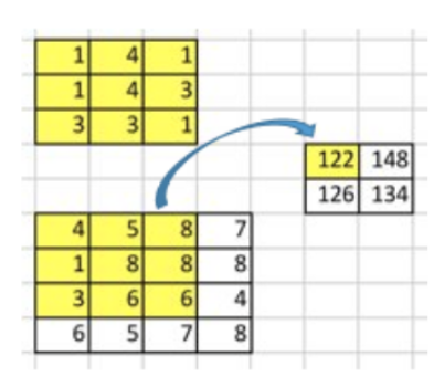
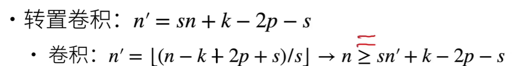
FCN 转置卷积实现尺寸变大,也有最近邻插值,双线性插值(初始化核)
卷积 :一群值转化为一个值的关系
轻松理解转置卷积(transposed convolution)或反卷积(deconvolution)_lanadeus-CSDN博客_转置卷积
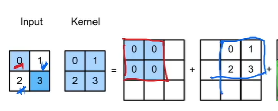
转置卷积: 原来一个值转化为一群值的对应关系,值上与原来无关(从信息论的角度看,卷积是不可逆的.所以这里说的并不是从output矩阵和kernel矩阵计算出原始的input矩阵.而是计算出一个保持了位置性关系的矩阵. )
超参数相同时,形状为逆变换
理解:填充k-p-1后, stride为将原矩阵在行列之间插s-1零行,再做传统卷积
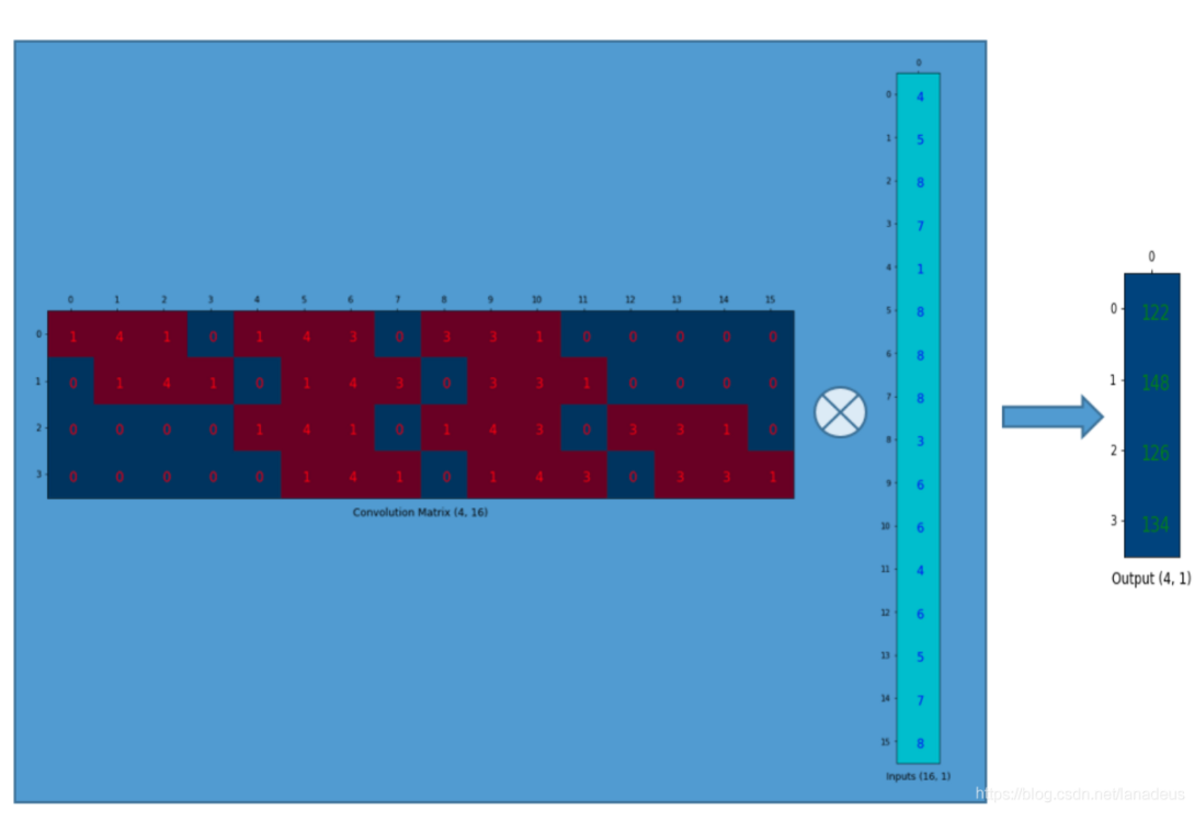
转置卷积的等价乘法矩阵 = 卷积核的乘法矩阵.T
1 2 d2l.corr2d(X, K) == torch.matmul(W, X.reshape(-1 )).reshape(2 , 2 )1 )).reshape(3 , 3 )
计算方法:1.相乘相加 2.倒转 扩充 正常卷积
FCN转置卷积: k-2p-s=0 双线性插值初始化
损失函数:直接cross_entropy ,分类维度在x的第二维度
1 2 3 x = torch.rand((32 , 21 , 320 ,480 ))32 , 320 , 480 )).long()
训练时,由于loss在一个batch上取平均值,比d2l小,所以要调大lr,否者会陷入局部最优 ,输出全黑
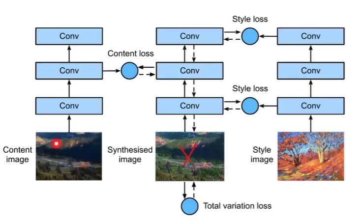
样式迁移 网络提取特征后,某些层上的特征相似 :gram矩阵 内容相似:直接对应位置MSE
内容特征深层次越好(忽略细节) [25] 风格特征多层结合[0, 5, 10, 19, 28]
风格矩阵:
对角线元素提供了不同特征图(a1,a2 … ,an)各自的信息,其余元素提供了不同特征图之间的相关信息。
contents_Y, styles_Y是提前准备好的。X为输入也是调整的对象,初始化为内容图img.weight.data.copy_(X.data)
迭代:
1 2 3 4 5
loss: 分为3部分, 内容(均方差)、风格(风格矩阵W *W.T的均方差)、平滑度损失
1 2 3 4 5 6 7 8 9 10 11 12 content_weight, style_weight, tv_weight = 1 , 1e3 , 10 def compute_loss (X, contents_Y_hat, styles_Y_hat, contents_Y, styles_Y_gram ):for Y_hat, Y in zip (for Y_hat, Y in zip (sum (10 * styles_l + contents_l + [tv_l]) return contents_l, styles_l, tv_l, l
大图片迁移:用小图迁移后,放大然后作为起始
牛仔行头检测 样本不平衡
 L2=0
L2=0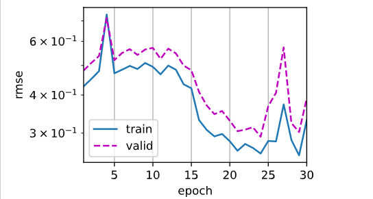
 batchsize128